
This article is about single-variable quadratic equations and their solutions. For more general information about the single-variable case, see Quadratic function. For the case of more than one variable, see Quadric.

The quadratic formula for the roots of the general quadratic equation
Because the quadratic equation involves only one unknown, it is called "univariate". The quadratic equation only contains powers of x that are non-negative integers, and therefore it is a polynomial equation, and in particular it is a second degree polynomial equation since the greatest power is two.
Quadratic equations can be solved by a process known in American English as factoring and in other varieties of English as factorising, by completing the square, by using the quadratic formula, or by graphing. Solutions to problems equivalent to the quadratic equation were known as early as 2000 BC
Solving the quadratic equation

Figure 1. Plots of quadratic function y = ax2 + bx + c, varying each coefficient separately while the other coefficients are fixed (at values a = 1, b = 0, c = 0)
Factoring by inspection
It may be possible to express a quadratic equation ax2 + bx + c = 0 as a product (px + q)(rx + s) = 0. In some cases, it is possible, by simple inspection, to determine values of p, q, r, and s that make the two forms equivalent to one another. If the quadratic equation is written in the second form, then the "Zero Factor Property" states that the quadratic equation is satisfied if px + q = 0 or rx + s = 0. Solving these two linear equations provides the roots of the quadratic.For most students, factoring by inspection is the first method of solving quadratic equations to which they are exposed.[2]:202–207 If one is given a quadratic equation in the form x2 + bx + c = 0, the sought factorization has the form (x + q)(x + s), and one has to find two numbers q and s that add up to b and whose product is c (this is sometimes called "Vieta's rule"[3] and is related to Vieta's formulas). The more general case where a does not equal 1 can require a considerable effort in trial and error guess-and-check, assuming that it can be factored at all by inspection.
Except for special cases such as where b = 0 or c = 0, factoring by inspection only works for quadratic equations that have rational roots. This means that the great majority of quadratic equations that arise in practical applications cannot be solved by factoring by inspection.[2]:207
Completing the square
Main article: Completing the square

Figure 2. For the quadratic function y = x2 − x − 2, the points where the graph crosses the x-axis, x = −1 and x = 2, are the solutions of the quadratic equation x2 − x − 2 = 0.

- Divide each side by a, the coefficient of the squared term.
- Rearrange the equation so that the constant term c/a is on the right side.
- Add the square of one-half of b/a, the coefficient of x, to both sides. This "completes the square", converting the left side into a perfect square.
- Write the left side as a square and simplify the right side if necessary.
- Produce two linear equations by equating the square root of the left side with the positive and negative square roots of the right side.
- Solve the two linear equations.


Quadratic formula and its derivation
Main article: Quadratic formula
Completing the square can be used to derive a general formula for solving quadratic equations, called the quadratic formula.[5] The mathematical proof will now be briefly summarized.[6] It can easily be seen, by polynomial expansion, that the following equation is equivalent to the quadratic equation:

A number of alternative derivations can be found in the literature. These proofs are simpler than the standard completing the square method, represent interesting applications of other frequently used techniques in algebra, or offer insight into other areas of mathematics.
Reduced quadratic equation
It is sometimes convenient to reduce a quadratic equation to an equation involving two instead of three constant coefficients. This is done by simply dividing both sides by a, which is possible because a is non-zero. This produces the reduced quadratic equation:[8]
It follows from the quadratic formula that the solution to the reduced quadratic equation is

Discriminant

Figure 3. Discriminant signs

- If the discriminant is positive, then there are two distinct roots
-
- both of which are real numbers. For quadratic equations with rational coefficients, if the discriminant is a square number, then the roots are rational—in other cases they may be quadratic irrationals.

- If the discriminant is zero, then there is exactly one real root
-
- sometimes called a repeated or double root.

- If the discriminant is negative, then there are no real roots. Rather, there are two distinct (non-real) complex roots[10]
-
- which are complex conjugates of each other. In these expressions i is the imaginary unit.

Geometric interpretation

Trajectory of the cliff jumper follows a shape of parabola, that is because horizontal displacement is a linear function of time( ), while vertical displacement is a quadratic function of time (
 ). As a result path follows quadratic equation
  , where v_x and v_y are horizontal and vertical components of the original velocity, a is gravity and h is original height.
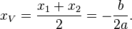
), while vertical displacement is a quadratic function of time (). As a result path follows quadratic equation , where v_x and v_y are horizontal and vertical components of the original velocity, a is gravity and h is original height. , and the y-coordinate of the vertex may be found by substituting this x-value into the function. The y-intercept is located at the point (0, c).
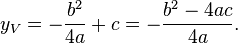
The solutions of the quadratic equation ax2 + bx + c = 0 correspond to the roots of the function f(x) = ax2 + bx + c, since they are the values of x for which f(x) = 0. As shown in Figure 2, if a, b, and c are real numbers and the domain of f is the set of real numbers, then the roots of f are exactly the x-coordinates of the points where the graph touches the x-axis. As shown in Figure 3, if the discriminant is positive, the graph touches the x-axis at two points; if zero, the graph touches at one point; and if negative, the graph does not touch the x-axis.
Quadratic factorization
The term


Graphing for real roots

Figure 4. Graphing calculator computation of one of the two roots of the quadratic equation 2x2 + 4x − 4 = 0. Although the display shows only five significant figures of accuracy, the retrieved value of xc is 0.732050807569, accurate to twelve significant figures.
Being able to use a graphing calculator to solve a quadratic equation requires the ability to produce a graph of y = f(x), the ability to scale the graph appropriately to the dimensions of the graphing surface, and the recognition that when f(x) = 0, x is a solution to the equation. The skills required to solve a quadratic equation on a calculator are in fact applicable to finding the real roots of any arbitrary function.
Since an arbitrary function may cross the x-axis at multiple points, graphing calculators generally require one to identify the desired root by positioning a cursor at a "guessed" value for the root. (Some graphing calculators require bracketing the root on both sides of the zero.) The calculator then proceeds, by an iterative algorithm, to refine the estimated position of the root to the limit of calculator accuracy.
Avoiding loss of significance
Although the quadratic formula provides what in principle should be an exact solution, it does not, from a numerical analysis standpoint, provide a completely stable method for evaluating the roots of a quadratic equation. If the two roots of the quadratic equation vary greatly in absolute magnitude, b will be very close in magnitude to , and the subtraction of two nearly equal numbers will cause loss of significance or catastrophic cancellation. A second form of cancellation can occur between the terms b2 and −4ac of the discriminant, which can lead to loss of up to half of correct significant figures.[7][13]
History
Babylonian mathematicians, as early as 2000 BC (displayed on Old Babylonian clay tablets) could solve problems relating the areas and sides of rectangles. There is evidence dating this algorithm as far back as the Third Dynasty of Ur.[14] In modern notation, the problems typically involved solving a pair of simultaneous equations of the form:

- Compute half of p.
- Square the result.
- Subtract q.
- Find the square root using a table of squares.
- Add together the results of steps (1) and (4) to give x. This is essentially equivalent to calculating

In 628 AD, Brahmagupta, an Indian mathematician, gave the first explicit (although still not completely general) solution of the quadratic equation ax2 + bx = c as follows: "To the absolute number multiplied by four times the [coefficient of the] square, add the square of the [coefficient of the] middle term; the square root of the same, less the [coefficient of the] middle term, being divided by twice the [coefficient of the] square is the value." (Brahmasphutasiddhanta, Colebrook translation, 1817, page 346)[15]:87 This is equivalent to:

The Jewish mathematician Abraham bar Hiyya Ha-Nasi (12th century, Spain) authored the first European book to include the full solution to the general quadratic equation.[26] His solution was largely based on Al-Khwarizmi's work.[21] The writing of the Chinese mathematician Yang Hui (1238–1298 AD) is the first known one in which quadratic equations with negative coefficients of 'x' appear, although he attributes this to the earlier Liu Yi.[27] By 1545 Gerolamo Cardano compiled the works related to the quadratic equations. The quadratic formula covering all cases was first obtained by Simon Stevin in 1594.[28] In 1637 René Descartes published La Géométrie containing the quadratic formula in the form we know today. The first appearance of the general solution in the modern mathematical literature appeared in an 1896 paper by Henry Heaton.[29]
Advanced topics
Alternative methods of root calculation
Vieta's formulas
Main article: Vieta's formulas

Figure 5. Graph of the difference between Vieta's approximation for the smaller of the two roots of the quadratic equation x2 + bx + c = 0 compared with the value calculated using the quadratic formula. Vieta's approximation is inaccurate for small b but is accurate for large b. The direct evaluation using the quadratic formula is accurate for small b with roots of comparable value but experiences loss of significance errors for large b and widely spaced roots. The difference between Vieta's approximation versus the direct computation reaches a minimum at the large dots, and rounding causes squiggles in the curves beyond this minimum.


This situation arises commonly in amplifier design, where widely separated roots are desired to ensure a stable operation (see step response).
Trigonometric solution
In the days before calculators, people would use mathematical tables—lists of numbers showing the results of calculation with varying arguments—to simplify and speed up computation. Tables of logarithms and trigonometric functions were common in math and science textbooks. Specialized tables were published for applications such as astronomy, celestial navigation and statistics. Methods of numerical approximation existed, called prosthaphaeresis, that offered shortcuts around time-consuming operations such as multiplication and taking powers and roots.[12] Astronomers, especially, were concerned with methods that could speed up the long series of computations involved in celestial mechanics calculations.It is within this context that we may understand the development of means of solving quadratic equations by the aid of trigonometric substitution. Consider the following alternate form of the quadratic equation,
[1]

where the sign of the ± symbol is chosen so that a and c may both be positive. By substituting
[2]

and then multiplying through by cos2θ, we obtain
[3]

Introducing functions of 2θ and rearranging, we obtain
[4]

[5]

where the subscripts n and p correspond, respectively, to the use of a negative or positive sign in equation [1]. Substituting the two values of θn or θp found from equations [4] or [5] into [2] gives the required roots of [1]. Complex roots occur in the solution based on equation [5] if the absolute value of sin 2θp exceeds unity. The amount of effort involved in solving quadratic equations using this mixed trigonometric and logarithmic table look-up strategy was two-thirds the effort using logarithmic tables alone.[30] Calculating complex roots would require using a different trigonometric form.[31]
- To illustrate, let us assume we had available seven-place logarithm
and trigonometric tables, and wished to solve the following to
six-significant-figure accuracy:
-

- A seven-place lookup table might have only 100,000 entries, and computing intermediate results to seven places would generally require interpolation between adjacent entries.


 (rounded to six significant figures)

Solution for complex roots in polar coordinates
If the quadratic equation with real coefficients has two complex roots—the case where
  requiring a and c to have the same sign as each other—then the solutions for the roots can be expressed in polar form as[32]
 and
and 
Geometric solution

Figure 6. Geometric solution of ax2 + bx + c = 0 using Lill's method. Solutions are −AX1/SA, −AX2/SA
Generalization of quadratic equation
The formula and its derivation remain correct if the coefficients a, b and c are complex numbers, or more generally members of any field whose characteristic is not 2. (In a field of characteristic 2, the element 2a is zero and it is impossible to divide by it.)The symbol

Characteristic 2
In a field of characteristic 2, the quadratic formula, which relies on 2 being a unit, does not hold. Consider the monic quadratic polynomial


In the case that b ≠ 0, there are two distinct roots, but if the polynomial is irreducible, they cannot be expressed in terms of square roots of numbers in the coefficient field. Instead, define the 2-root R(c) of c to be a root of the polynomial x2 + x + c, an element of the splitting field of that polynomial. One verifies that R(c) + 1 is also a root. In terms of the 2-root operation, the two roots of the (non-monic) quadratic ax2 + bx + c are

This is a special case of Artin–Schreier theory.
Tidak ada komentar:
Posting Komentar